Where exactly are the people? Recovering 3D pedestrian tracks from a walking robot's logs
Back in 2025, I led the development of the ACME dataset, the largest by duration (currently Sep 2026) multi-cultural multi-embodiment social navigation dataset. We (Team NUS) collected data on the Unitree Go2 Platform. Our robot was equipped with a Intel RealSense D435i and Hesai XT-16 LiDAR for capturing the scene. Unfortunately post recording, we found that the depth data (which we recorded as Compressed ROS2 messages), was corrupted due a realsense driver bug.
This meant it was very hard to locate the pedestrians in 3D around the robot, an essential input modality for learning social navigation policies. I then spent quite some time trying different sensor fusion and depth estimation methods to retrieve the lost information, but ultimately found the results sub-par, primarily due to the sparsity of the LiDAR point clouds, the limited FOV and the poor POV of the robot, and poor depth estimation results. Even trained 3D pedestrian detection models performed poorly primarily due to dataset mismatch: most MoT models are trained on Autonomous Driving datasets with Dense LiDARs, with different object ranges and sensor setups.
Fast Forward to Sep 2026, I find the current depth-estimation models are far more performant and, of course (as is evident from the format of this post) CLAUDE is at my disposal to try out this side-project while I work on finishing up my PhD thesis. So this post (mostly written by claude and editted by me), is a step-by-step tutorial on how I (+CLAUDE obv) retrieved much better 3D pedestrian tracking around the robot from limited noisy starting data and using a variety of different off-the-shelf models, heuristics and sensor-fusion. I’ll make the code available at some point.
How we turned camera detections, odometry and a sparse lidar on a quadruped robot into 360°, identity-consistent 3D pedestrian tracks, and the mistakes that taught us the most along the way.
The robot’s walk, seen from above at 2× speed. Before: camera detections combined with estimated metric depth: people only inside the camera’s view, in a drifting odometry frame. After: 360° pedestrian predictions around the robot, with a stable identity, on a map from which the people have been removed.
All figures come from one recording in our go2nus dataset: 44 seconds of a Unitree Go2 trotting along a busy campus walkway, past a group of people standing and chatting, with a steady stream of people walking in both directions.
1. What we started with
Each recording comes from sensors mounted on the robot:
- a forward-facing Intel RealSense D435i RGB-D camera, with person detections and tracks from REGROUP (YOLO with the BoT-SORT tracker), and person segmentation masks;
- the robot’s onboard odometry, from its legs and IMU;
- a Hesai XT-16 LiDAR (16 beams, 10 Hz), mounted about half a metre above the ground.
The D435i records depth as well, but due to the depth corruption, every bit of distance information had to come from the lidar, or be estimated from the colour images.
The camera feed at 1.5× speed, with the tracker’s boxes and the lidar scan projected into the image, coloured by distance (people are blurred for privacy). The lidar is sparse: only a handful of beams cross each person.
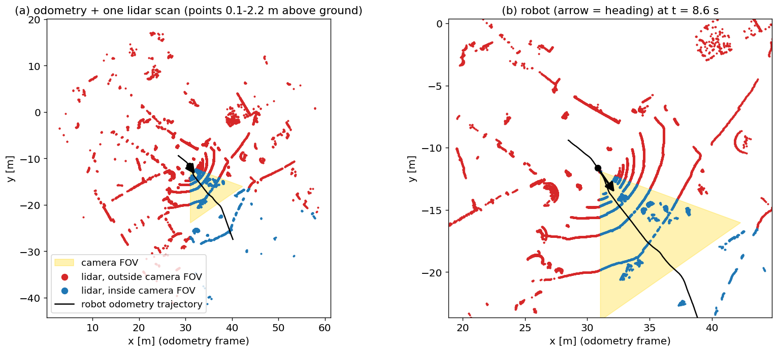 One moment from above: the lidar sees all around the robot, the camera only a wedge in front.
The question is simple: where is each person, in metres, at every moment? Boxes tell us who and in which direction, but not how far.
2. Camera-side 3D:
Our first pipeline, estimates each detected person’s position from the camera side. With the camera’s own depth unusable, it combines every other depth cue available inside the person’s mask:
- lidar: the lidar points that fall inside the mask;
- VGGT-Ω: dense metric depth predicted from the image sequence;
- VGGT, range-corrected and lidar-anchored: the same depth, corrected for its bias with distance and rescaled per track to agree with the lidar;
- Video Depth Anything: monocular video depth, for comparison.
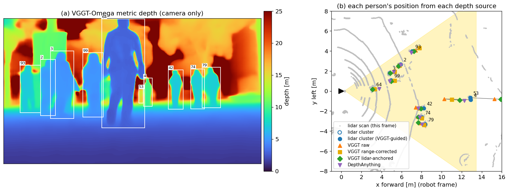 One frame: the VGGT-Omega depth map (left) and, from above, where each depth source places each person (right).
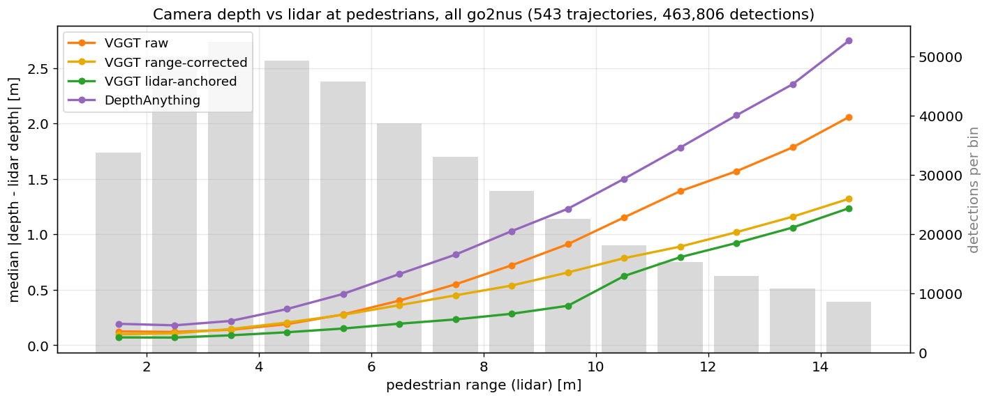 How far camera depth is from the lidar, by distance, over the whole dataset.
Camera depth is excellent up close and degrades quickly with distance, which is why the lidar matters, so we must combine the two, each weighted by how much it can be trusted at that range: camera depth helps pick the right lidar points when several people overlap, and the lidar fixes the camera depth’s scale. Each track is then smoothed over time, with outliers down-weighted and short gaps filled.
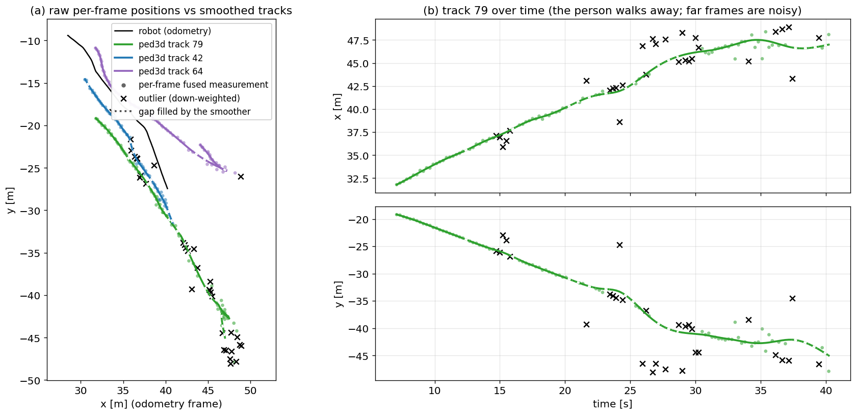 Per-frame positions (dots) and the smoothed tracks (lines). The person in green walks away from the robot; far away, single-frame positions scatter, and the smoother keeps the track on course.
This gave good positions inside the camera’s field of view. Three problems remained:
- positions were expressed in the robot’s odometry frame, which drifts;
- nothing was known about people beside or behind the robot (outside camera FOV but within lidar range);
- track identities churned: one person walking past produced several short fragemented tracks due to REID errors.
3. Fixing the frame: offline SLAM
We ran an offline lidar SLAM on every recording: KISS-ICP for scan matching, and a GTSAM pose graph that keeps the map level using the tilt (roll and pitch) from the robot’s own odometry, plus smoothing of the trotting gait.
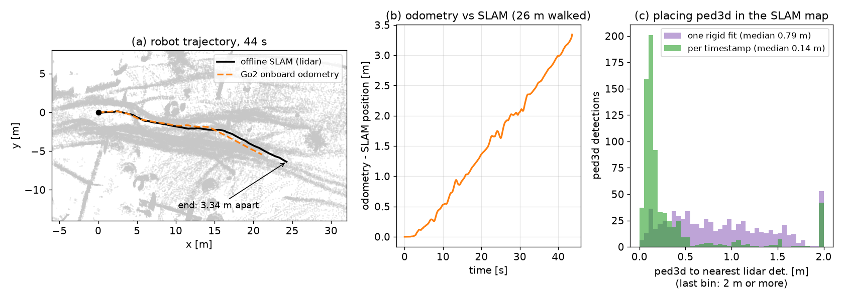 (a) The robot’s odometry against the SLAM trajectory; (b) the gap between them over time; (c) how well pedestrian positions line up with the lidar when moved into the SLAM map in two different ways.
Over a 26 m walk, the odometry drifts about 3 m away from the SLAM trajectory, and the error keeps growing, so no single transform between the two frames can fix it. What works is re-projecting at every timestamp: take the pedestrian back into the robot’s frame using the odometry at that moment, then place it using the SLAM pose at that same moment. The drift cancels out, and only the robot-to-person offset, which the camera and lidar measure well, remains.
4. A map without people
To find people all around the robot with the lidar, we first need to know what the world looks like without them. Stacking every scan into one map gives ghost trails:
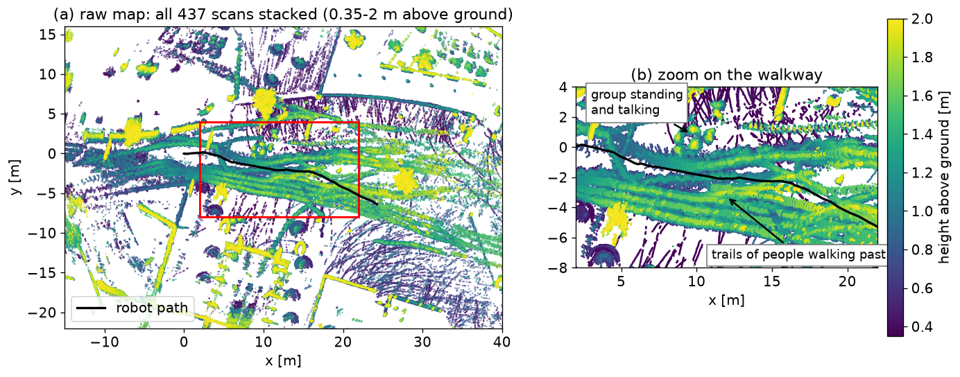 The raw accumulated map, coloured by height: every walker leaves a smear along the walkway, and the standing group shows up as solid blobs.
We used ERASOR2, a dynamic-object removal method (with Patchwork++ ground segmentation and HDBSCAN clustering as its inputs), and went one step further: points belonging to people tracked in the previous step are removed from each scan before ERASOR2 runs.
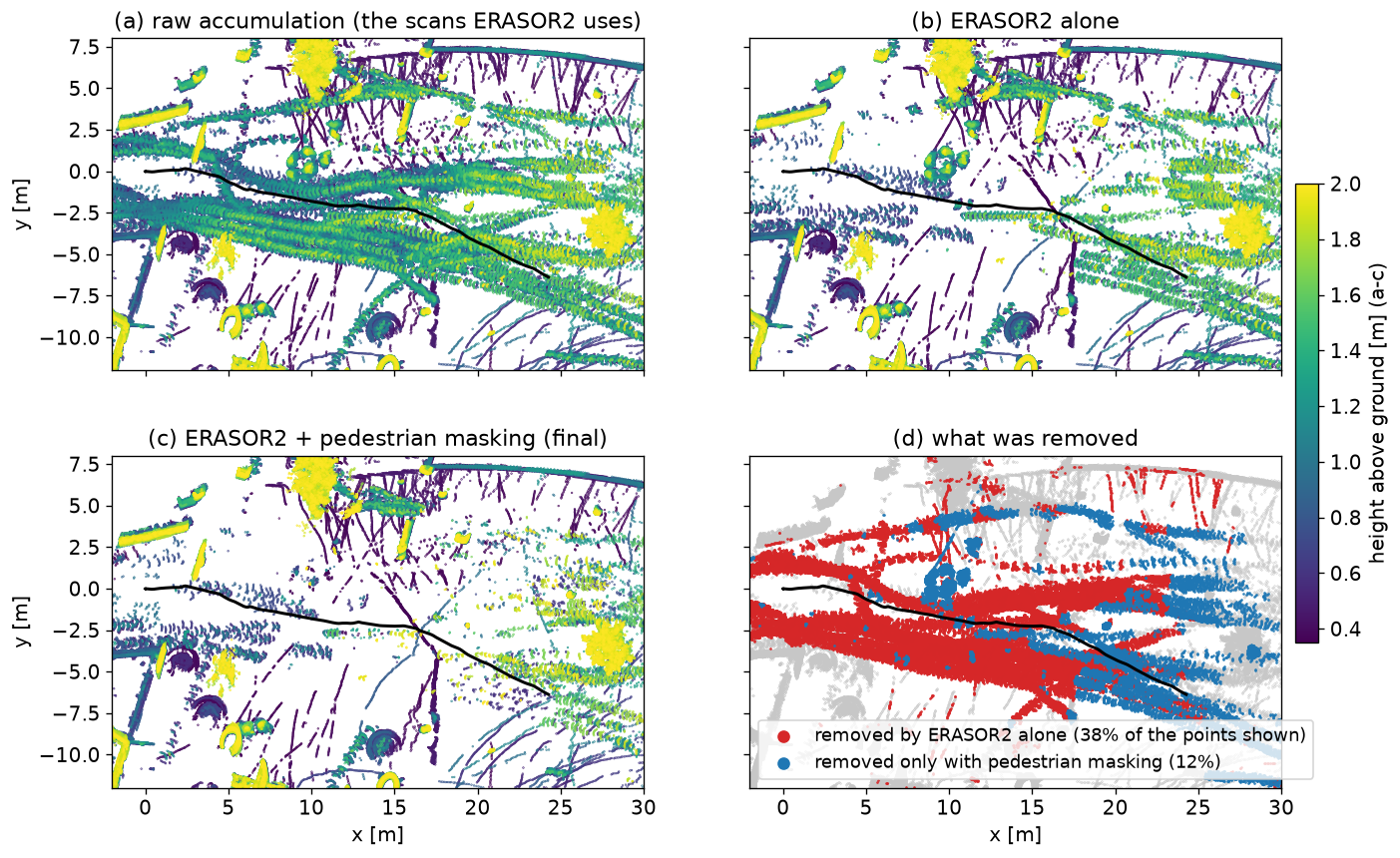 The stacked scans (a), ERASOR2 alone (b), ERASOR2 with pedestrian masking (c), and what was removed (d): red by ERASOR2 alone, blue only once tracked pedestrians were masked.
Lesson 1: a clean run is not a correct run. Our first attempt finished without errors, produced a tidy-looking map, and removed almost nothing. ERASOR2 needs to see the ground to judge what’s moving, and a setting copied from a car-mounted lidar excluded the ground for our low-mounted one. Only measuring what had been removed revealed it.
Lesson 2: people standing still are the hard case. For much of the recording, a group of people stand chatting by the walkway. To ERASOR2 they look like static objects.
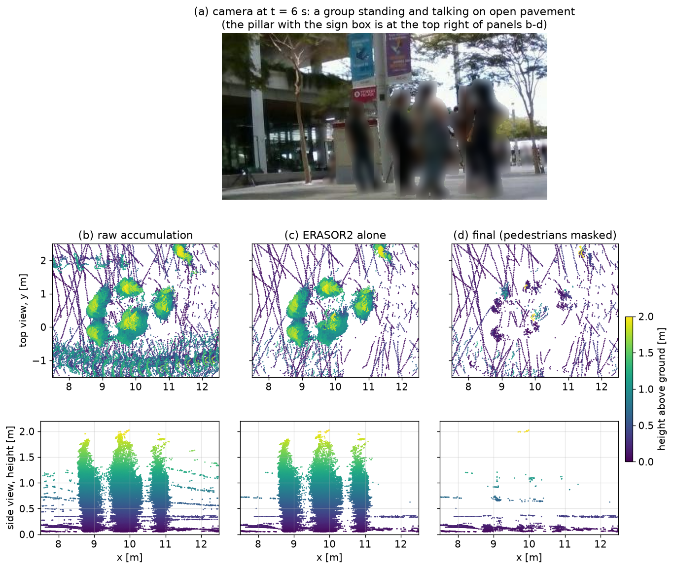 The standing group in the camera (top), and around them in the map, from above and from the side (bottom): raw, ERASOR2 alone, and final.
The fix: once the camera detects a person standing still, we assume they stay where they were last seen, and remove the lidar points at that spot in every scan until the end of the recording before building the map. The camera loses them as soon as the robot walks past, but the lidar keeps seeing them, and they’re still there twenty seconds later. This only cleans the map: the pedestrian tracks we output contain only positions that were actually observed.
5. 360° detection: subtracting the map
With a clean map, finding people in a scan becomes simple: anything that isn’t in the map has moved. For each scan we remove the ground and everything the map explains, group what’s left, and keep the clusters that are the size of a person. Of course the assumption here is that anything moving and within the constraints of our clusters is likely a pedestrian.
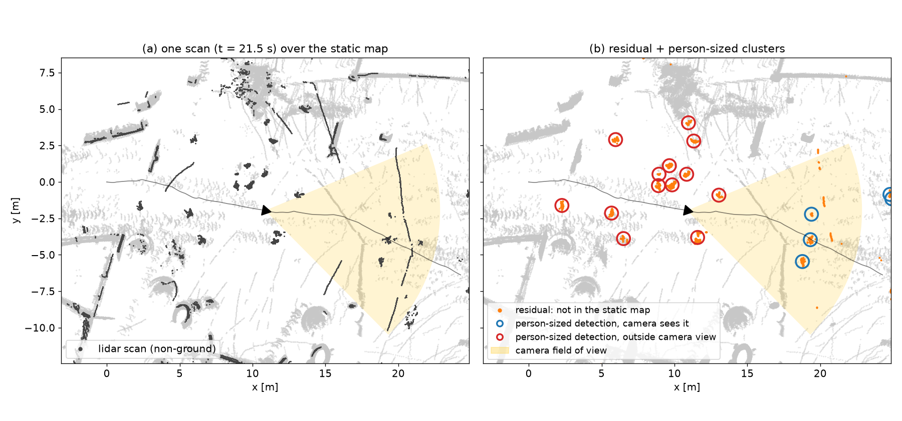 One scan over the static map (left), and what’s left after subtracting the map (right): person-sized detections in blue where the camera can see them, red where it can’t. The cluster behind the robot is the standing group.
No trained lidar detector is needed: the map already removes the lamp posts and planters that a shape-based detector would mistake for standing people. Where the camera can check it, this finds the large majority of the people the camera sees, within about 15 cm.
6. Tracking: from greedy links to a Kalman filter
Our first lidar tracker simply linked each detection to the nearest recent one, and tracks broke apart constantly. We replaced it with a standard multi-target tracker: a constant-velocity Kalman filter, globally optimal matching between tracks and detections, and a smoothing pass that fills gaps and re-joins broken tracks.
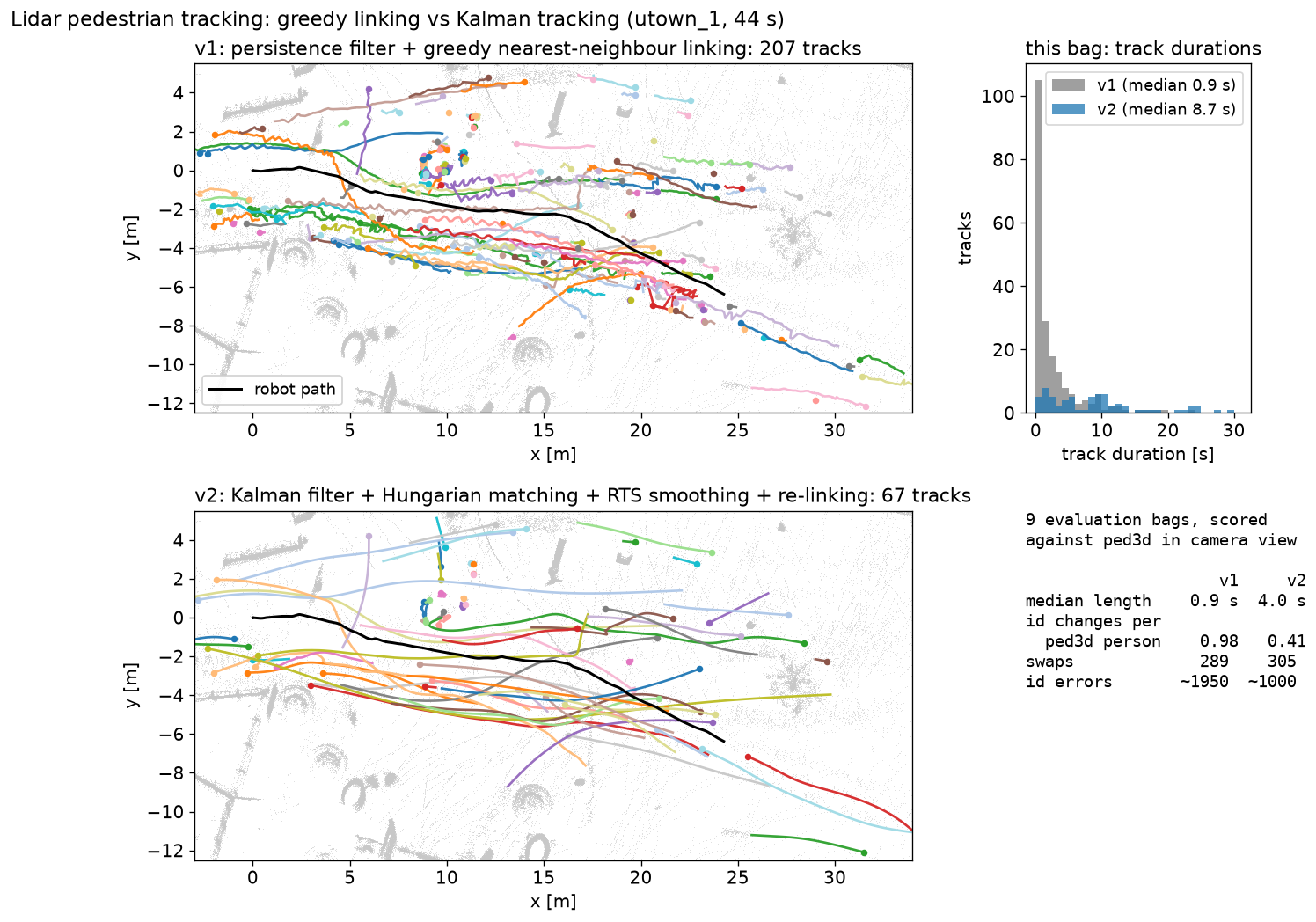 Greedy linking (top) against the Kalman tracker (bottom); each colour is one track. The same people, far fewer and far longer tracks.
Across our evaluation recordings, tracks became about four times longer and identity errors roughly halved.
7. One set of tracks: fusing camera and lidar
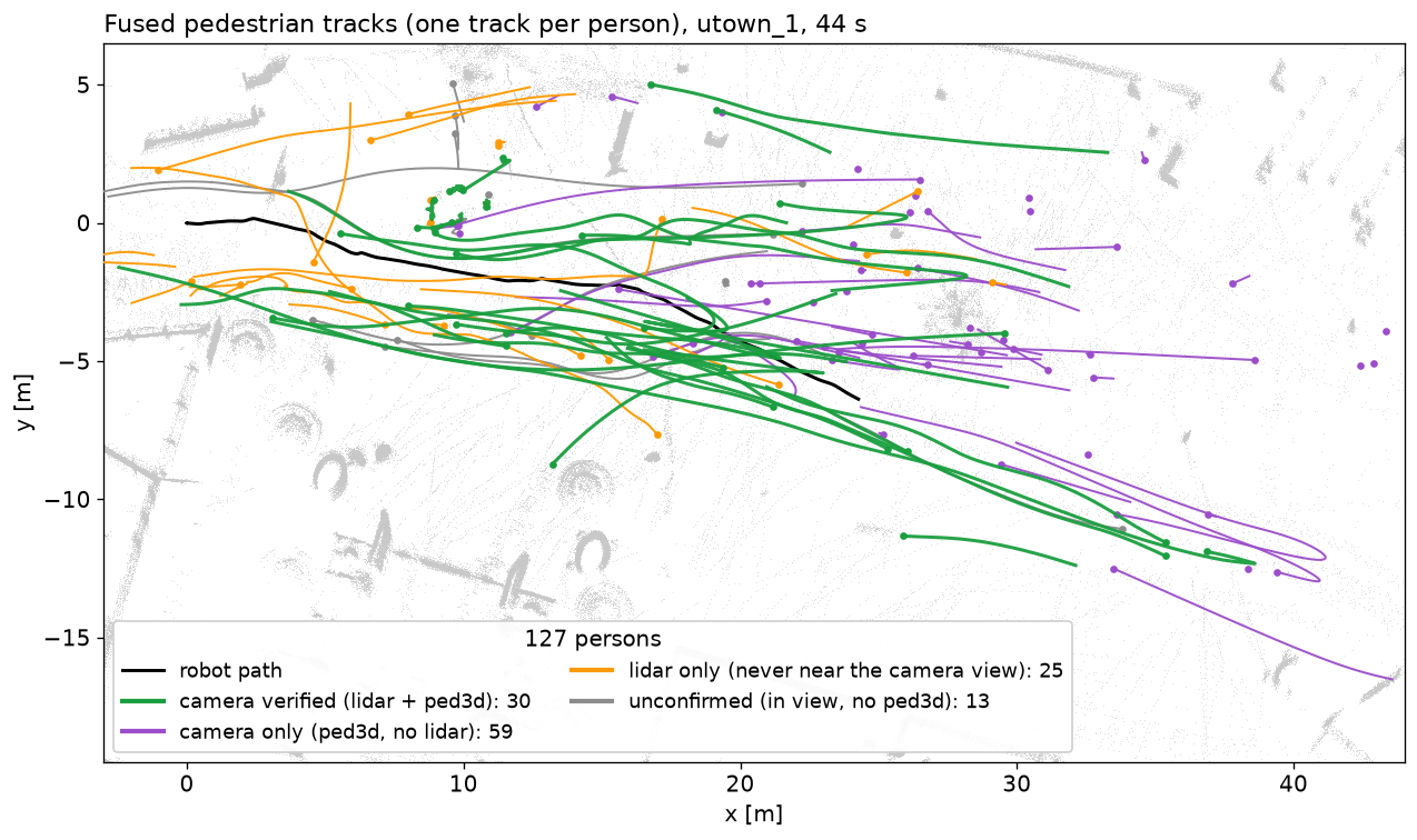
We now had two sets of tracks: camera (camera + depth estimated) and lidar (all around the robot, ten times a second), with unrelated identities. The fusion:
- matches lidar tracks to camera tracks frame by frame;
- repairs swaps: if a lidar track jumps from one camera-identified person to another, it is cut there;
- groups tracks into people, joining camera’s fragments through the lidar and the lidar’s gaps through camera, but never merging two tracks that are far apart at the same moment;
- combines measurements without counting anything twice: camera’s position already contains the lidar, so we only add its camera-depth part, plus its lidar part where our lidar tracker missed the person;
- smooths each person’s track and labels them: seen by both sensors, camera only, lidar only, or unconfirmed (near the camera but never recognised as a person: bikes, carts, foliage).
Lesson 3: agree on what “position” means. camera reports the centre of a person’s body; our lidar detections reported the centre of the visible surface, which is a steady ~10 cm closer to the robot. Once both used the body centre, the two sources agreed to within about 8 cm.
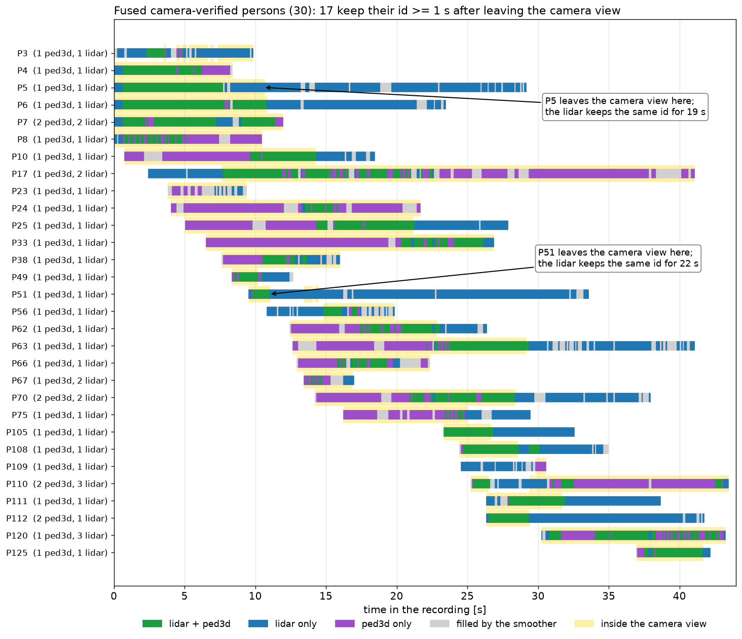 Each row is one person seen by both sensors; colour shows which sensor observed them, yellow shading marks when they were in the camera’s view. More than half keep their identity well after leaving it: P5 walks out of view at 10 s and is followed on the lidar alone for another 19 s.
Does the camera also make positions more accurate where the lidar already sees someone? We checked by hiding stretches of lidar detections: not noticeably. The camera’s real contribution is identity and coverage: confirming that a lidar blob is a person, stitching fragments together, fixing swaps, and covering people the lidar misses.
9. More places, same picture
The same before-and-after, on three more recordings from very different settings, each at 2× speed.
An outdoor event at UTown, the most crowded recording in the dataset. The camera sees about a dozen people at a time; around the robot there are around fifty.
Indoors, walking through the crowd at the RoboSG event hall.
A busy walkway by the Science faculty, with people streaming past on both sides of the robot.
10. Where this leaves us
Limits. Someone who stands still for an entire recording and is never detected becomes part of the map, and is invisible to the lidar. Outside the camera’s view, a lidar identity swap can’t be corrected. Close to the robot, the lidar’s narrow vertical field of view cuts off people’s heads.
What we’d tell ourselves at the start:
- Look at the camera image before naming an object from a point cloud.
- A clean run and a plausible-looking result are not evidence: measure what the step actually did.
- Before fusing two sources, check that they measure the same thing.
- Don’t let a clever safeguard override the evidence the pipeline was built to use.
11. A by-product: maps without people
Every recording also leaves behind a clean map of the place the robot walked through, with the people taken out. Turned into a 2D navigation map, it marks what the robot could bump into (black), where it has seen that the way is clear (white), and what it never saw (grey). Because only points that survive pedestrian removal count as obstacles, the people who were walking around during the recording leave no trace: the walkways come out clear.
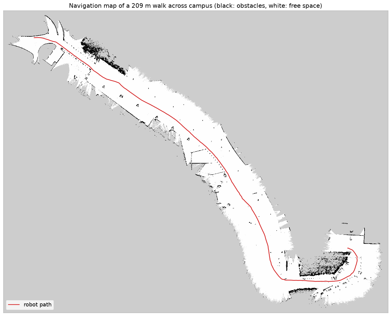 The longest walk in the dataset, a little over 200 m across campus.
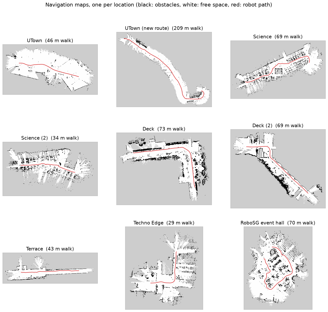 One map per location in the dataset, from campus walkways and covered decks to an indoor event hall.
Tools we used
- REGROUP, Ultralytics YOLO and BoT-SORT: person detection, segmentation and tracking in the images
- VGGT-Ω: metric depth from the image sequence
- Video Depth Anything: monocular depth baseline
- KISS-ICP and GTSAM: offline lidar SLAM
- ERASOR2, Patchwork++ and HDBSCAN: dynamic-object removal from the lidar maps
- ros2_leg_detector: the 2D-laser baseline in section 8
- Nav2: the occupancy-grid map format of section 11